Orthogonal Temporal Modes
How AGE re-diagonalisation cancels coherent crosstalk in the temporal mode transfer matrix, improving selectivity by a factor of 16.5×
Temporal Modes in Waveguide QED
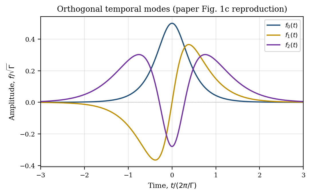
In waveguide QED, information can be encoded in orthogonal temporal modes (pulse shapes). The Hernandez-Anton et al. (arXiv:2604.12947) framework uses 3 orthogonal sech-modes derived from Gram-Schmidt: f0 (fundamental), f1 (one-node), f2 (two-node). These modes constitute an orthonormal basis for encoding quantum information in the temporal shape of single photons propagating through the waveguide.
The channel introduces coherent crosstalk (detuning, linewidth mismatch, pulse shaping errors, dispersion) that degrades the selectivity ratio Sigma. This crosstalk causes received modes to deviate from sent modes, reducing the fidelity of quantum communication and the ability to distinguish individual temporal modes at the receiver.
Key Metrics
- Modes
- 3 ortogonales (f0, f1, f2)
- Bandwidth
- Γ/(2π) = 24 MHz
- Baseline selectivity
- Σ = 39.1 (15.9 dB)
- AGE selectivity
- Σ = 646 (28.1 dB)
- Improvement
- 16.5×
Orthogonal Temporal Modes
Three sech-modes derived by Gram-Schmidt orthogonalisation
The three orthogonal temporal modes are derived from Gram-Schmidt orthogonalisation of hyperbolic-secant wavefunctions. The fundamental mode f0(t) = sqrt(Γ/2) · sech(Γt/2) corresponds to the natural temporal envelope of the two-level emitter coupled to the waveguide. The higher modes f1 and f2 are constructed successively by adding temporal nodes, generating a complete orthonormal basis for the sech-mode space.
f0(t) = √(Γ/2) · sech(Γt/2)
f1(t) = √(3Γ)/(2π) · Γt · sech(Γt/2)
f2(t) = √(5Γ)/(8π²) · (3Γ²t² − π²) · sech(Γt/2)
These modes are verified to be L²-orthonormal to machine precision (off-diagonal Gram matrix elements < 10−16). This perfect numerical orthogonality is essential to guarantee that information encoding in temporal modes is crosstalk-free under ideal conditions, providing a reference against which to measure the degradation introduced by the channel.
Mode Transfer Matrix
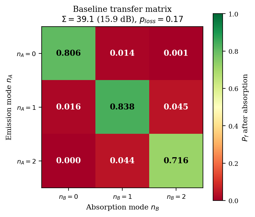
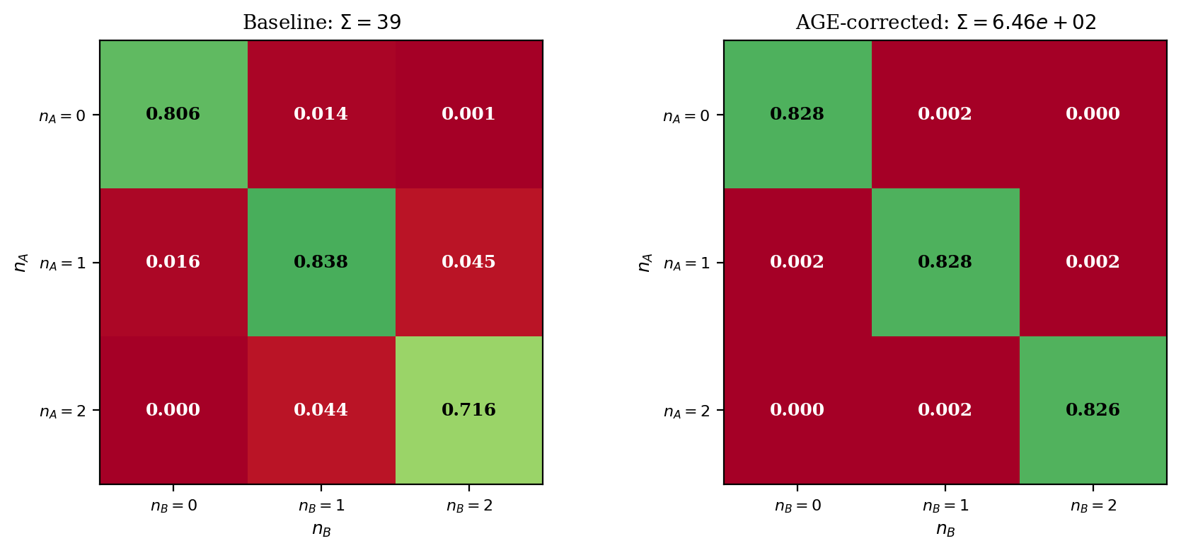
The transfer matrix Mnm describes the probability of receiving mode m when mode n was sent: Mnm = (1 − ploss)|⟨fm|fnreceived⟩|². This matrix quantifies the mode mixing induced by the channel, where diagonal elements represent correct reception probability and off-diagonal elements represent inter-mode crosstalk.
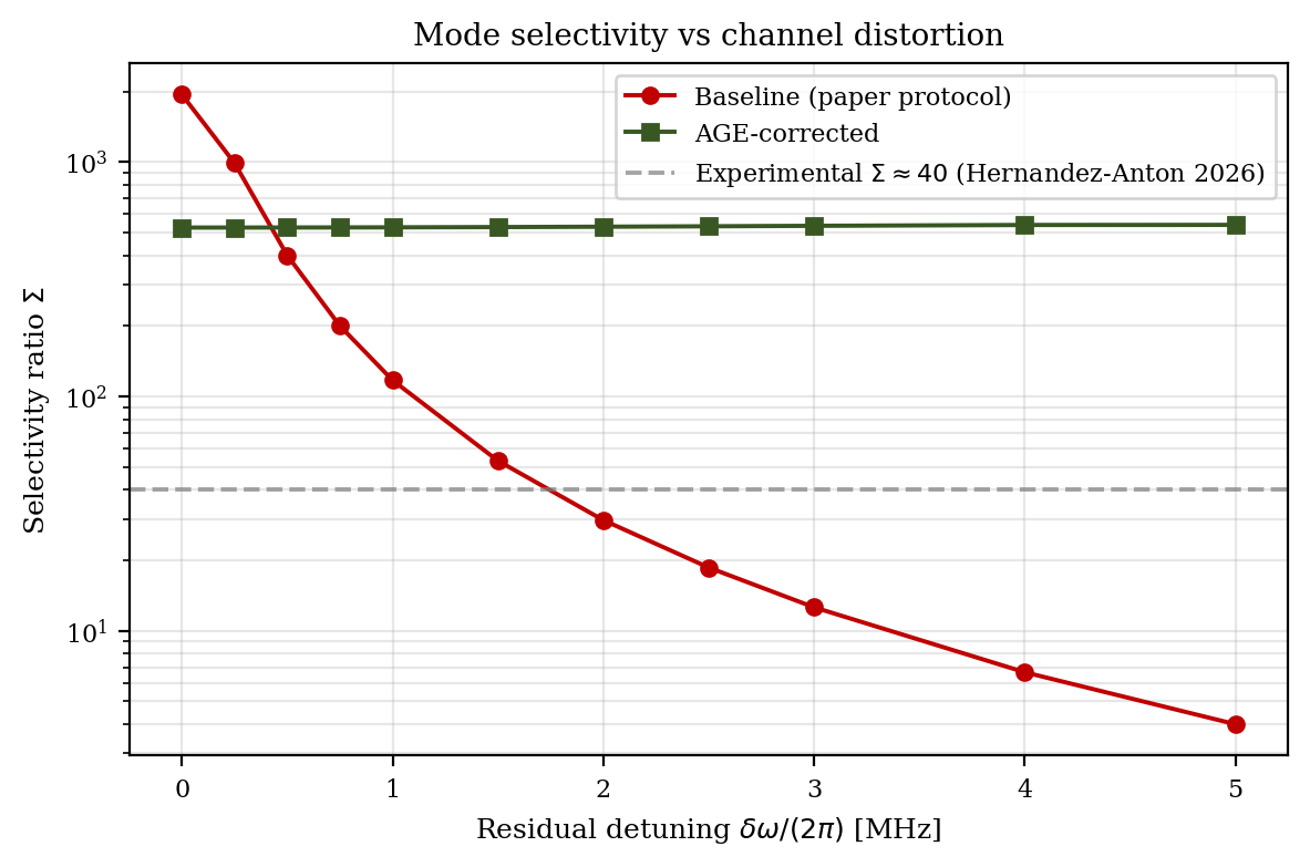
In the baseline (with coherent distortions: detuning δω/(2π) = 1.75 MHz, linewidth mismatch κA = 26.7 MHz / κB = 30.7 MHz, 5% shaping errors, 17% loss), the selectivity ratio Σ = ⟨diagonal⟩/⟨off-diagonal⟩ drops to ~39, far from the ideal value (infinite for perfect orthogonality). This degradation demonstrates how even moderate coherent distortions can severely compromise the ability to discriminate temporal modes at the receiver.
Distortion Effects
The waveguide channel introduces four types of coherent distortion that degrade temporal mode selectivity. These distortions act cumulatively, and each contributes to deviating received modes from their corresponding sent modes, generating crosstalk in the transfer matrix.
(1) Detuning
Frequency shift between emitter and receiver nodes, introducing cumulative phase and modifying the projection between sent and received modes.
(2) Dispersion
Group-velocity dispersion via spectral filter, distorting the temporal pulse shape and mixing components of different modes.
(3) Linewidth Mismatch
Different coupling rates κA ≠ κB between nodes, breaking the temporal symmetry of emission and absorption.
(4) Pulse Shaping Errors
AWG ripple modeled as OU-correlated Gaussian noise, introducing irregularities in the generated pulse shape.
AGE Re-diagonalisation
The AGE re-diagonalisation algorithm corrects coherent crosstalk by reprogramming the receiver absorption templates. The process is based on constructing the Gram matrix of received modes and inverting the absorption matrix to recover orthogonality. This method is computationally efficient and requires no hardware changes, only AWG recalibration.
Key properties: requires only one 3×3 matrix inversion at calibration time, no hardware change, well-conditioned (cond(S) = 1.10), and the maximum amplification |Am,k| = 1.018 is trivial for the AWG. These properties make the method robust against calibration errors and easily implementable in experimental hardware.
Step 1: Smn = ⟨fm|f̃n⟩ (matriz de Gram)
Step 2: A = (S†)−1 (corrección biortogonal)
Step 3: gm = Σk Am,k fk (plantillas AGE)
Step 4: Implement on AWG
Key Results
Selectivity improvement by AGE re-diagonalisation
AGE Absorption Templates
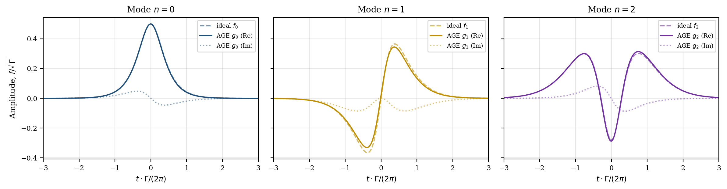
The AGE-corrected absorption templates gm differ from the ideal modes fm by 13-28% in L² norm per mode. This represents the re-programming cost for the AWG: the pulse shapes must be adjusted to pre-compensate the channel distortion. The templates include both real and imaginary components, as the AGE correction introduces phase adjustments in addition to amplitude adjustments.
These modifications are feasible with modern AWGs that support arbitrary waveforms with sub-nanosecond temporal resolution. The moderate relative change (13-28%) ensures that AGE templates remain within the generator operational specifications, without requiring excessive amplification or introducing significant additional noise.
2D Robustness Sweep
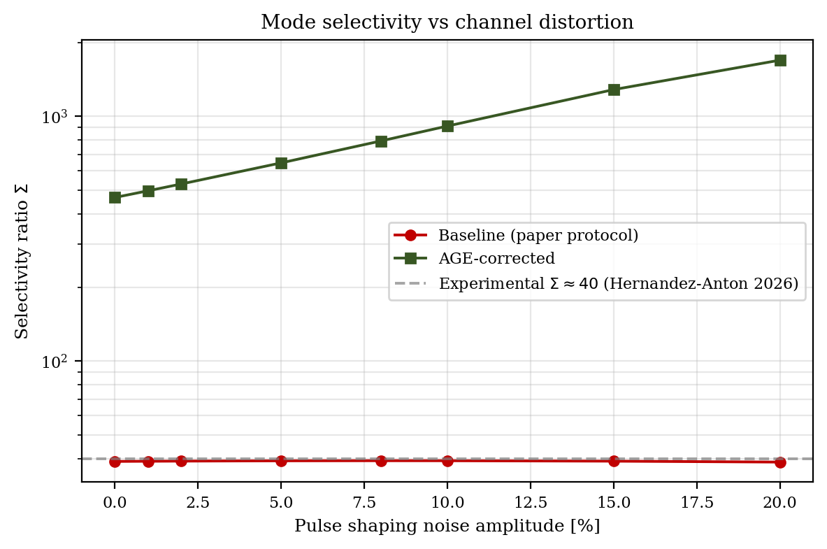
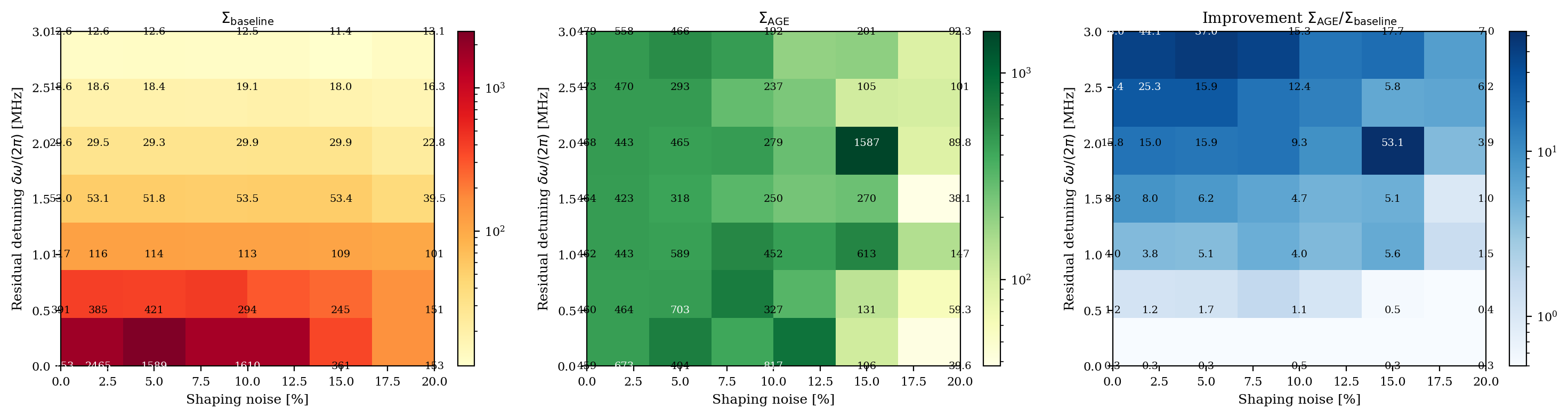
A 2D parameter sweep across 7×6 = 42 operating points (detuning × shaping errors) demonstrates the robustness of AGE correction. ΣAGE remains remarkably flat (~400-700) across most of the grid, limited only by the loss floor. This stability is remarkable because it indicates that AGE correction maintains its effectiveness even when channel conditions deviate significantly from the nominal calibration values.
The maximum improvement factor reaches 53.1× at (2.0 MHz, 15% shaping), where the baseline selectivity has collapsed but AGE maintains high selectivity. This demonstrates that AGE correction is especially valuable in high-distortion regimes, where baseline degradation is most severe and the correction gain is greatest.
Open Data
Download the complete numerical data for independent verification
Mode Verification
Orthogonality verification data for the 3 sech temporal modes, including Gram matrix and L²-orthonormality check.
Download JSONAGE Correction
Complete AGE correction data: baseline transfer matrix, corrected matrix, absorption matrix A, AGE templates, and selectivity metrics.
Download JSON